[![PyPi][pypi-shield]][pypi-url]
[![PyPi][pypiversion-shield]][pypi-url]
[![PyPi][downloads-shield]][downloads-url]
[![License][license-shield]][license-url]
[pypi-shield]: https://img.shields.io/pypi/pyversions/pina-mathlab?style=for-the-badge
[pypi-url]: https://pypi.org/project/pina-mathlab/
[pypiversion-shield]: https://img.shields.io/pypi/v/pina-mathlab?style=for-the-badge
[downloads-shield]: https://img.shields.io/pypi/dm/pina-mathlab?style=for-the-badge
[downloads-url]: https://pypi.org/project/pina-mathlab/
[codecov-shield]: https://img.shields.io/codecov/c/gh/zenml-io/zenml?style=for-the-badge
[codecov-url]: https://codecov.io/gh/zenml-io/zenml
[contributors-shield]: https://img.shields.io/github/contributors/zenml-io/zenml?style=for-the-badge
[contributors-url]: https://github.com/othneildrew/Best-README-Template/graphs/contributors
[license-shield]: https://img.shields.io/github/license/mathLab/pina?style=for-the-badge
[license-url]: https://github.com/mathLab/PINA/blob/main/LICENSE.rst
[linkedin-shield]: https://img.shields.io/badge/-LinkedIn-black.svg?style=for-the-badge&logo=linkedin&colorB=555
[slack-shield]: https://img.shields.io/badge/-Slack-black.svg?style=for-the-badge&logo=linkedin&colorB=555
[slack-url]: https://zenml.io/slack-invite
[build-shield]: https://img.shields.io/github/workflow/status/zenml-io/zenml/Build,%20Lint,%20Unit%20&%20Integration%20Test/develop?logo=github&style=for-the-badge
[build-url]: https://github.com/zenml-io/zenml/actions/workflows/ci.yml

Solve equations, intuitively.
A simple framework to solve difficult problems with neural networks.
Explore the docs »
🏁 Table of Contents
- Introduction
- Quickstart
-
Solve Your Differential Problem
- Contributing and Community
- License
# 🤖 Introduction
🤹 PINA is a Python package providing an easy interface to deal with *physics-informed neural networks* (PINN) for the approximation of (differential, nonlinear, ...) functions. Based on Pytorch, PINA offers a simple and intuitive way to formalize a specific problem and solve it using PINN.
- 👨💻 Formulate your differential problem in few lines of code, just translating the mathematical equations into Python
- 📄 Training your neural network in order to solve the problem
- 🚀 Use the model to visualize and analyze the solution!
# 🤸 Quickstart
[Install PINA](https://mathlab.github.io/PINA/_rst/installation.html) via
[PyPI](https://pypi.org/project/pina-mathlab/). Python 3 is required:
```bash
pip install "pina-mathlab"
```
# 🖼️ Solve Your Differential Problem
PINN is a novel approach that involves neural networks to solve supervised learning tasks while respecting any given law of physics described by general nonlinear differential equations. Proposed in [Physics-informed neural networks: A deep learning framework for solving forward and inverse problems involving nonlinear partial differential equations](https://www.sciencedirect.com/science/article/pii/S0021999118307125?casa_token=p0BAG8SoAbEAAAAA:3H3r1G0SJ7IdXWm-FYGRJZ0RAb_T1qynSdfn-2VxqQubiSWnot5yyKli9UiH82rqQWY_Wzfq0HVV), such framework aims to solve problems in a continuous and nonlinear settings.
## 🔋 1. Formulate the Problem
First step is formalization of the problem in the PINA framework. We take as example here a simple Poisson problem, but PINA is already able to deal with **multi-dimensional**, **parametric**, **time-dependent** problems.
Consider:
$$
\begin{cases}
\Delta u = \sin(\pi x)\sin(\pi y)\quad& \text{in}\, D \\
u = 0& \text{on}\, \partial D \end{cases}$$
where $D = [0, 1]^2$ is a square domain, $u$ the unknown field, and $\partial D = \Gamma_1 \cup \Gamma_2 \cup \Gamma_3 \cup \Gamma_4$, where $\Gamma_i$ are the boundaries of the square for $i=1,\cdots,4$. The translation in PINA code becomes a new class containing all the information about the domain, about the `conditions` and nothing more:
```python
class Poisson(SpatialProblem):
output_variables = ['u']
spatial_domain = Span({'x': [0, 1], 'y': [0, 1]})
def laplace_equation(input_, output_):
force_term = (torch.sin(input_.extract(['x'])*torch.pi) *
torch.sin(input_.extract(['y'])*torch.pi))
nabla_u = nabla(output_.extract(['u']), input_)
return nabla_u - force_term
def nil_dirichlet(input_, output_):
value = 0.0
return output_.extract(['u']) - value
conditions = {
'gamma1': Condition(Span({'x': [-1, 1], 'y': 1}), nil_dirichlet),
'gamma2': Condition(Span({'x': [-1, 1], 'y': -1}), nil_dirichlet),
'gamma3': Condition(Span({'x': 1, 'y': [-1, 1]}), nil_dirichlet),
'gamma4': Condition(Span({'x': -1, 'y': [-1, 1]}), nil_dirichlet),
'D': Condition(Span({'x': [-1, 1], 'y': [-1, 1]}), laplace_equation),
}
```
## 👨🍳 2. Solve the Problem
After defining it, we want of course to solve such a problem. The only things we need is a `model`, in this case a feed forward network, and some samples of the domain and boundaries, here using a Cartesian grid. In these points we are going to evaluate the residuals, which is nothing but the loss of the network.
```python
poisson_problem = Poisson()
model = FeedForward(layers=[10, 10],
output_variables=poisson_problem.output_variables,
input_variables=poisson_problem.input_variables)
pinn = PINN(poisson_problem, model, lr=0.003, regularizer=1e-8)
pinn.span_pts(20, 'grid', ['D'])
pinn.span_pts(20, 'grid', ['gamma1', 'gamma2', 'gamma3', 'gamma4'])
pinn.train(1000, 100)
plotter = Plotter()
plotter.plot(pinn)
```
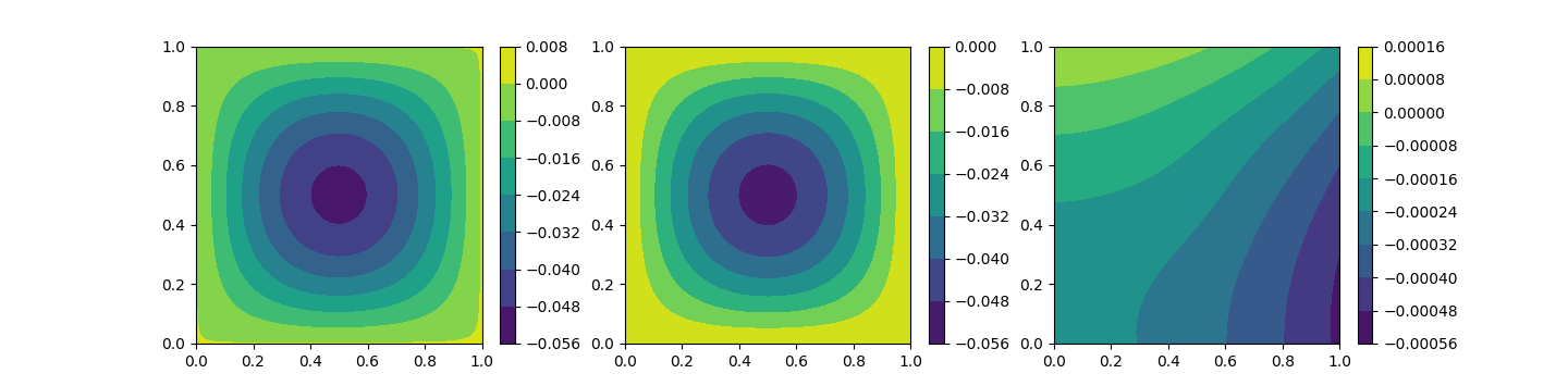
After the training we can infer our model, save it or just plot the PINN approximation. Below the graphical representation of the PINN approximation, the analytical solution of the problem and the absolute error, from left to right.
# 🙌 Contributing and Community
We would love to develop PINA together with our community! Best way to get
started is to select any issue from the [`good-first-issue`
label](https://github.com/mathLab/PINA/issues?q=is%3Aopen+is%3Aissue+label%3A%22good+first+issue%22). If you
would like to contribute, please review our [Contributing
Guide](CONTRIBUTING.md) for all relevant details.
We warmly thank all the contributors that have supported PINA so far:
 Made with [contrib.rocks](https://contrib.rocks).
# 📜 License
PINA is distributed under the terms of the MIT License.
A complete version of the license is available in the [LICENSE.rst](LICENSE.rst) file in this repository. Any contribution made to this project will be licensed under the MIT License.
Made with [contrib.rocks](https://contrib.rocks).
# 📜 License
PINA is distributed under the terms of the MIT License.
A complete version of the license is available in the [LICENSE.rst](LICENSE.rst) file in this repository. Any contribution made to this project will be licensed under the MIT License.